2. Intro to Analytica

This section provides an introduction to Analytica, as it relates to the iAM.AMR project.

Other Analytica resources are available, including first-party documentation. If you’re a collaborator, you also have access to recorded sessions in the iAM.AMR Team Repo (GitHub login required).

2.1. Basic Concepts in Analytica

An Analytica model consists of one or more objects. An Analytica object, much like a physical object, has a form (it occupies space), and is characterized by its attributes, such as its name (title), its identifier, its class, and its definition. Each of these attributes contains one or more values; values, whether they are text strings, numbers, or formulae, are the data that modellers and users enter into the model.

The most common object in Analytica is the node (the terms object and node are often, though incorrectly, used interchangeably), and the most important attribute of each node is its definition. The definition is where quantitative data is stored, and where the mathematical relationships between nodes are defined. Other attributes generally contain qualitative data or descriptors (metadata), such as units of measurement.

An influence diagram – the interface you see when you open the model – is a collection of nodes and their connections which serve to communicate the underlying mathematical relationships captured in the model. Because these models are designed to be accessible to users, it is essential that they are as clear and understandable as possible.

2.1.1. Node Types

Analytica has ten different types of nodes, which we differentiate into two groups: basic and complex. The basic nodes (variable, chance, objective, and constant) are, for the most part, functionally equivalent. Analytica differentiates between these node types (by default colour and shape) solely to convey information to users; generally, a chance node contains a probability distribution, an objective node contains a model output relevant to users, a constant node contains an immutable constant (such as Avogadro’s number), and a variable node contains any data not belonging to one of the aforementioned categories. The choice between these node types is largely stylistic.

The upshot of this principle, is that while Analytica will in some instances automatically select a node type, modellers may coerce a basic node to any other basic node type which they believe is appropriate. In contrast, the complex nodes (module, index, function, text, and button) each confer distinct and unique properties, and are therefore are only useful in specific situations. Where applicable, they are described in subsequent sections.

2.1.2. Attributes

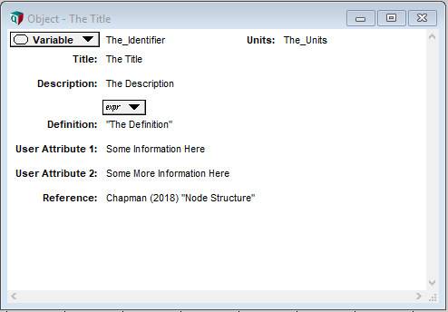
Each object in Analytica is described by a series of attributes; the minimum set of attributes required to describe an object include the title, the identifier, and the definition.

The title is a non-unique string that appears as a label for the object in an influence diagram. The identifier is a unique, non-space-containing string used to identify or reference the object in functions, formulae, and definitions of subsequent objects. The definition is the content of the object –- the main repository for data and data manipulation.

Comparing Analytica to a traditional spreadsheet program, the title is equivalent to a label beside a cell, the identifier is equivalent to the cell name (e.g. B4), and the definition is equivalent to the cell content (e.g. “dog”, 18, or “=C4+D4”).

2.1.3. Identifier

An object’s identifier is a unique, non-space-containing string used to identify or reference the object in functions, formulae, and definitions of subsequent objects. Analytica automatically generates this identifier using the title provided; identifiers are limited to 20 characters, cannot start with a number, and cannot contain punctuation or spaces.

For example, a node with the title “Frequency Tree” will automatically be given the identifier “Frequency_Tree”. Similarly, a node with the title “Jim’s Favourite Cookies” will automatically be given the truncated identifier “Jim_s_Favourite_Cook”. Where the generated identifier is already in use, a non-padded number will be appended to the identifier (i.e. a subsequently created node with the title “Frequency Tree” will be assigned the identifier “Frequency_Tree1”. In the event the resulting numbered identifier exceeds 20 characters, the title is further truncated (i.e. a subsequently created node with the title “Jim’s Favourite Cookies” will be assigned the identifier “Jim_s_Favourite_Coo1”).

Note that while capitalization of identifiers is preserved within the definitions and formulae of the model, identifiers are not case-sensitive.

2.1.3.1. Lucid Influence Diagrams and Best Practices

Lumina has coined the phrase ‘Lucid Influence Diagrams’ to describe diagrams that follow best practices, and clearly and effectively communicate purpose to users and modellers alike. Several key recommendations from the Analytica Wiki are reproduced here. Of course, none of these are hard and fast rules; use your discretion when applying these conventions, and construct your diagrams as they best make sense to you (and of course, as they best serve your stakeholders’ needs).

2.1.4. Node Titles

Nodes should include descriptive, but succinct titles. Use common abbreviations where appropriate, but balance these choices against usability. For example, a node describing the probability of antimicrobial resistance at retail is better represented as “Prob. Resistance at Retail” than the more succinct, but difficult to understand “Prob. Res. Ret.”.

2.1.5. Node identifiers

Recall that the title of each node (shown by default in the user interface) is distinct from its identifier. A node’s identifier is the true designator of the node – it is the string used to identify the node in functions, formulae, and definitions of subsequent nodes. This identifier can (and should be) more succinct than the title, as it will be repeatedly entered elsewhere in the model (and used solely by model builders, who have a more thorough understanding of the model).

As node identifiers are automatically created, they may be nonsensical or unnecessarily complex. Using our former example, if we had several nodes titled “Jim’s Favourite Cookies” (perhaps within a model of several bakeries), we could easily end up with a series of identifiers “Jim_s_Favourite_Coo1, Jim_s_Favourite_Coo2, Jim_s_Favourite_Coo3” and no idea as to which bakeries these refer.

Therefore, it is best practice to manually edit the identifier after it is generated, using a uniform and consistent naming scheme (e.g. “Jim_Fav_BakeryA”, “Jim_Fav_BakeryB”). The schema developed for the iAM.AMR project is described in the conventions.

Tip

If you are updating the titles of nodes, you can disable the automatic prompt to regenerate the identifier based on the new title in the preferences menu –- this can speed up the process of updating the model where the identifier has already been set correctly.

2.1.6. Visual Consistency

Colour, size, and node type can be used to communicate information to the user, but only when these attributes are used consistently. Nodes containing similar data or which perform a similar function should be the same size and shape – larger or more colourful nodes suggest importance and draw attention.

Likewise, the large-scale arrangement of the influence diagram communicates information to the user; influence diagrams tell a story with their structure, and should flow as one would expect – from left-to-right and from top-to-bottom. Nodes should be aligned where possible to reduce visual clutter; horizontal and vertical arrows, which do not intersect, are easier to follow than their askew or tangled counterparts.

Arrows between nodes can be supressed using individual node style properties (by right-clicking the node, and selecting node style). This is recommended where relationships are implied by positioning or title, and suppression of the links reduce visual clutter. Arrow suppression is especially useful when implementing a User Defined Function (UDF) – the function node will be visually linked to all objects in which the function is called unless output arrows from the function node are disabled.

The text-case used in node titles (and identifiers) should be consistent across the model. While title-case may be more attractive for short titles, sentence case improves readability. Decide on one format, and use it consistently throughout the model.

The schema developed for the iAM.AMR project is described in the conventions.

2.1.7. Attributes and Metadata

Recall that the minimum set of attributes required to describe an object include the title, the identifier, and the definition. However, Analytica also includes a number of built in attributes to capture metadata, such as the description and unit fields, which should always be completed where possible. Notably, modellers can create their own attributes (or enable lesser-known built-in attributes) to further document their models or add functionality; the attributes panel is available under the object menu in the menu bar.

The built-in Cell Default attribute specifies the value assigned to newly-created cells. This attribute, enabled on a per-node or model-wide basis, replaces Analytica’s default cell value of zero. Setting this attribute is useful where zero values may result in errors during evaluation (e.g. the node is used as a divisor), where the cell is a complex function, of when the cell is otherwise cumbersome to regularly update (e.g. a series of choice functions in a table).

The built-in OnChange attribute, enabled on a per-node basis, specifies an expression to be evaluated or action to be taken any time the definition of the node changes. Importantly, expressions in the OnChange attribute are able to affect changes throughout the model (i.e. global assignment) that are otherwise disallowed by Analytica (other than through a button action). Specifying an OnChange attribute is useful for input validation, or synchronizing multiple nodes.

2.1.7.1. Indices and Array Abstraction

2.1.8. Indices

Indices are lists, consisting of text strings, non-sequential numbers, or number series, which act as strata for data throughout a model. The simplest way of thinking of an index is as containing the row or column labels of a table – indices delineate data into categories, across which comparisons can be drawn. An example of a simple index is a list of months, which serves as the row or column labels for a table containing data collected on a monthly basis.

When defining a list, Analytica presents three options: a list, a list of labels, and a sequence. A list may contain any type of data (string, numeric, etc.). A list of labels can only contain strings – any data entered will be coerced to a string. A sequence is a list of numbers that do not need to be individually specified; where a large list of regularly incremented numbers is required, a sequence is a great shortcut (e.g. a list of numbers from 1 to 100).

2.1.9. Array Abstraction

Indices serve as the basis for Analytica’s ‘Intelligent Array’ system, one of Analytica’s most powerful functions. For those readers with experience in programming, array abstraction (Lumina’s terminology for the implementation of the Intelligent Array system) is akin to automatic vectorization of code. In simpler terms, any operation applied to a table or function which includes an index, is automatically applied over the entire index. Let’s return to our example of an index containing a list of months; multiplying a table containing monthly sales data (indexed by the Month Index) by 5 will automatically multiply each cell by 5 –- no need to specify the operation for each individual cell.

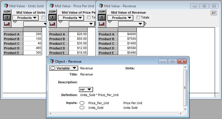
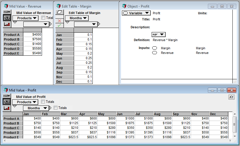
The true power of array abstraction however, is Analytica’s ability to match indices, and automatically propagate these indices throughout the model. Let’s look at a different example; calculating the revenue associated with multiple products. Given two tables, containing the number of units sold, and the price per unit, we can calculate the revenue per product with a single multiplicative operation. The number of units for Product A in the first table is multiplied by the price of Product A in the second table (and so on for all products), and the result is a single column table, also indexed by the product names.

Additionally, Analytica can identify where operations occur over two different indices and automatically create a matrix, populated with the cross product of those indices. Expanding on our previous example, we can calculate the profit on each product throughout the year, assuming our profit margin changes as a result of material cost (perhaps we’re a bakery, and the cost of vanilla changes throughout the year). Given two tables, containing the revenue per product, and the margin per month, we can calculate our profit again with a single multiplicative operation. The revenue for each product is automatically multiplied by each month’s margin value, and the result is a matrix, indexed both by product names and months.

The rules of array abstraction will become more apparent as you build your models; array abstraction (and the rules that govern it) are some of the more difficult concepts to grasp in Analytica, especially before you’ve had an opportunity to try it yourself. One key thing to remember is that indices are propagated forward in the model, and each index adds a dimension to your table or matrix. Any operation on an object associated with an index will bring that index forward into the calculation. The exception to this rule are array reducing functions; for example, Sum() adds elements of a table along an index (for example, if we wanted the total revenue for all products), reducing the dimensionality of the table by one (i.e. removing the index).

2.1.9.1. Decision Nodes and DetermTables

As you become more familiar with indices and the Intelligent Array system in Analytica, you may notice that the size of tables (and therefore their compute time) increases rapidly –- it’s very easy to build a model that will test the limits of your available computational resources. You may also realize that you require user input in the model, in the form of a choice between one or more scenarios.

2.1.10. Choice Functions and Decision Nodes

Decision nodes (and the Choice functions contained therein) address both of these facets of model building by presenting the user with a list of options, and allowing them to select one or all of these options – only these options are propegated through the model and evaluated. The easiest way to understand how Choice functions are implemented in Analytica is to look the corresponding code:

Choice(INDEX, POSITION, AllowAll)

All of the options presented to the user are specified in an INDEX. The simplest example of an index is one containing the labels “Yes” and “No”. When the user interacts with the choice node and makes a decision, the Choice function stores that decision as the POSITION of that element in the index. In our simple example, if the user chooses “Yes”, and “Yes” is the first element of the index, POSITION = 1; if the user chooses “No”, POSITION = 2. The importance of this concept to end-users is minimal, however model builders should be aware that we can change the user’s selection programmatically, by updating the POSITION argument of the Choice function. The final argument, AllowAll, is a logical, which specifies whether the user is allowed to choose all of the options, not just one.

2.1.11. DetermTables

Recall that an index can be thought of as the rows or columns of a table. What the Choice function actually does is take an existing index, perform a subset (i.e. select one element from the index), and returns that subset as an index. This means we can dynamically resize our tables based upon the choice of the user, reducing computational requirements, and returning data tailored to the user’s choices.

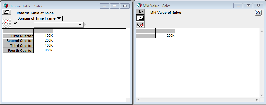
However, we can’t do this with a traditional Table in Analytica. As Analytica will remind you, if you ever go to delete an element from an index, data are lost as the Table shrinks. Instead, we rely on a DetermTable; an object which works exactly like a Table, but dynamically resizes when calculated. In the example shown below, the DetermTable is indexed by a Decision node, which is set to “Second Quarter”. This means that while the DetermTable contains all of the information necessary to evaluate the whole table, it will only evaluate and return the “Second Quarter” value.

If we wanted to achieve a similar effect using a standard Table, we would need to manually delete and re-add elements of the index, then repopulate the Table – not something that’d you’d want to do regularly. Moreover, it is not something that end-users could easily accomplish.

Tip

You can always use DetermTables in place of standard tables; there is seemingly no downside, and no reconfiguration is required if a Decision node is later included in the model.

2.1.12. A Note on implementation

There are two important things to consider when using a Choice function. The first is that a Choice function can be self-indexed (i.e. the index of choices is specified within the Decision node itself). We generally do not recommend that option, as the index will likely need to be re-used at some point, elsewhere within the model.

The second is that there is an additional step when configuring a Decision node using a Choice function with an external index (as described in the previous section). In addition to specifying the external index in the Choice function definition, it must also be specified as the Domain of the Decision node, in the Domain attribute. If the attribute is not specified, Analytica will throw an error. Note that if the Domain attribute is not accessible in the node window, enable the attribute as previously described.

2.2. Modules

Models get big fast.

This is particularly true of Analytica models, wherein data and model process are coupled to their layouts (recall, Lumina refers to this concept as an Influence Diagram). Accordingly, the Analytica wiki includes a section explicitly addressing working with large models.

In brief, Analytica models can be broken down into smaller parts, called modules. These modules fit together like puzzle pieces – each contains its own nodes and connections that together, form a whole. A given module can be shared among multiple models.

Within a model, modules are organized hierarchically, like folders on your desktop. You may have many modules in the root of your model, or choose to add modules within other modules. Or, if you prefer, you may just have one large model with no modules at all (but will be doing a lot of scrolling!). A module looks like a standard node, but you’ll be able to identify them by their thick black borders.

2.2.1. Types of Modules

Standard modules (or simply, modules) exist within the parent model file as a logical sub-dividion of your model. For example, you may add a user-interface at the root level of your model, and hide the actual model from view within a module (we do this in the iAM.AMR models). Or, you might put all nodes related to a particular antimicrobial class within a single class module.

Hint

‘Enter the model’ on the front page of each model is actually a module! We use modules throughout the iAM.AMR models to better organize information and improve user experience.

Filed modules exist within a seperate file (i.e. a seperate .ANA file), linked remotely to your parent model file. For example, you may have different filed modules for each animal species (that can be updated by a different subject-matter expert), that are all linked together in a single parent model.

Filed modules offer several important advantages, including re-use across multiple models, and improved collaboration (as everyone can work on their own section). However, it is important to note that you must have all of the files present to run the parent model.

Returning to our above example, if you have a parent model “agri-food production”, linked to seperate chicken, cattle, and swine filed modules, you must have all four to run the complete model. And, they must be stored/distributed in the same relative location (see below).

2.2.2. Linking Modules in Analytica

For a complete explanation of how to link filed modules to parent models in Analytica, see the Analytica Wiki. For a practical example, see the iAM.AMR.HUB section.

• Changes in a linked module (i.e. a filed module) are propegated in both directions. Do not make an edit within the module in your model that you do not want to propegate to all models linked to that module.
• Generally, you do not want to embed a module, as that breaks the link to the original module file, and no updates or changes will be propegated in either direction.
• For existing links, you will have to re-link the modules if the files have been moved relative to one another. For example, when you download the files from GitHub, you will have to re-link the module when open.

You can think of models and modules fitting together like puzzle pieces; similar models and modules ‘click’ into one another to form a whole.

Attention

As a result of this ‘pluggable’ framework, the iAM.AMR models are often distributed across multiple files – ensure you have all the files you need to run your model.