3. The Hub Module
3.1. countTable Data Format
Here, we define a countTotal table as a table of counts of positives, and of total observations of a trial, indexed by the CountTotal index at positions ‘Count’ and ‘Total’ respectively.
The purpose of a countTotal table is to store the number of positive observations and the number of total observations of a trial – across an arbitrary number of additional indices – in a standardized format, for manipulation using array operations. For example, directly calculating prevalence (Count / Total), or for use in a distribution (specifically the binomial distribution family, which considers the number of successes in a series of independent experiments). See the Math and Stats Section for more details.
Both the CIPARS-derived baseline probabilities of resistance, and the CIPARS-derived retail microbial recovery rate are specified as countTotal tables.
3.2. Baseline
The baseline data are stored as counts (as countTotal tables), or as prevalences, in separate tables for each microbe.
Why do we separate baseline data into tables by microbe? Or by any index for that matter – why not use one big table? Analytica supports – and is indeed designed for – highly dimensional tables, and we’ve extolled the virtue of Analytica’s Intelligent Array system throughout this documentation.
We separate them because these tables don’t actually share all of the same indices; the microbial sub-type index changes, depending on the microbe. Recall from our discussion of Analytica’s Intelligent Array system , that when presented with two different indices, Analytica will automatically array-abstract, and fill-in and compute values for each combination of index A and index B. If we were to include Salmonella and Campylobacter sub-types indices in the same table – for example – Analytica would create cells for the intersection of each of these indices, both the parent (i.e. Salmonella or Campylobacter), and the child (i.e. the subtype). The resultant table would have cells such as “Salmonella jejuni” or “Campylobacter Heidelberg”).
This seems simple enough to address (ignore nonsensical combinations), but each nonsensical slice of the table is replicated for each year, region, animal, and antimicrobial. So it’s not just “Salmonella jejuni”, but “Salmonella Enterica jejuni”, “Salmonella Heidelberg Jejuni”, and so on – this quickly becomes computationally prohibitive.
Tip
Often times, we may refer to arrays with multiple, non-congruent indices as “jagged’, because they aren’t of consistent size across each other index.
All of the available baseline data is taken from CIPARS surveillence data, available in the annual reports.
There is currently no baseline data directly specified as a prevalence.
3.3. Recovery Rate
To Do.
3.4. Consumption Rates
To Do.
3.5. Population
To Do.
3.5.1. Included Functions
3.5.2. Model Documentation
The HUB is equipped with an Analytica library called Model Documentation. This library provides a way to export all descriptions and definitions for objects in your model to an Excel spreadsheet.
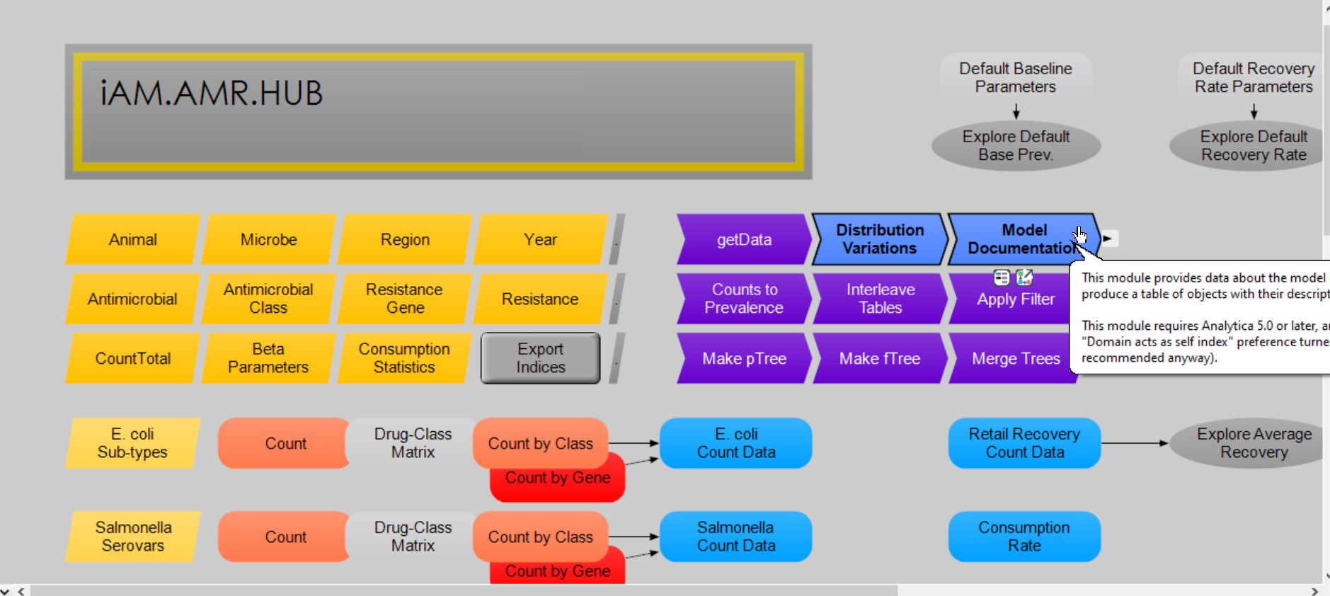
The iAM.AMR.HUB model, with the model documentation library highlighted
Detailed instructions for using this library can be found by clicking on the Model Documentation node (highlighted in the above figure) within the iAM.AMR.HUB itself.
Each function is described within its own Description attribute. Where necessary, further information is provided here.
3.6. Get Data
The Get Data function takes a table indexed by the baseline indices, and returns a subset of the data, filtered by the provided story-model indices.
Note
If a main-model index is omitted, the table will be returned indexed by the baseline index.
3.7. Count to Prevalence
The Count to Prevalence function converts a countTotal table into a table of prevalences, represented by a Beta distribution. For more details on the use of the Beta() distribution, see the Math and Stats section.
By default, the function replaces missing count and total values with ‘1’ and ‘15’ respectively. Alternatively, it can return ‘Null’, or a Beta() distribution specified with alternative default count and total values.
Important
The defaults specified here are not the direct parameters used in the Beta() distribution. See the Math and Stats section for more details.
3.8. Interleave
The Interleave function combines two similarly-indexed tables, overwriting data in <<originalData>> with <<newData>> where matched and available.
Note
Interleave() respects array abstraction; where <<newData>> is specified with fewer indices than <<originalData>>, <<newData>> is expanded (abstracted) to fit.
By default, Interleave() replaces all data for which there is a match (<<replaceMissing>> = True). To only replace existing data (i.e. replace existing data, not fillng data gaps), set (<<replaceMissing>> = False.
3.8.1. Depreciated Functions
To Do.
Important
The iAM.AMR.HUB module is the module to which the story models are linked. Do not link your story model to the iAM.AMR.HUB.GM module.
What does this mean in practice? To make changes to our Hub module, we first make the changes to the GM. Then, we save a protected copy, overwriting the existing production model. Because the name and location of the Hub module do not change, the story models automatically recognize the new production copy, and any changes are propagated when the story models are opened.
You can think of making changes to the Hub module like making changes to a manuscript. All changes are made in Microsoft Word, before creating a PDF to submit to the journal.